TLG Aerospace is Your Trusted Partner for CFD Services
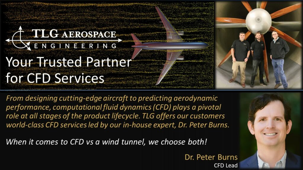
From designing cutting-edge aircraft to predicting aerodynamic performance, computational fluid dynamics (CFD) plays a pivotal role at all stages of the product lifecycle.
Since we were just in the wind tunnel last month (see our post here), we thought it would be fun to discuss how CFD can be used as a virtual wind tunnel. We’re big fans of real-world testing, but we think you get more value when you combine it with CFD-based predictions.
Below are a few of the advantages CFD has over a wind tunnel which make it a complementary tool.
◾ Upfront costs and schedule – Wind tunnel models are expensive and take time to build. These costs pay off once you are in the tunnel, but CFD has a much lower cost and lead time to seeing the first actionable results. Further, CFD allows teams to refine their early-stage concepts quickly, which means a design is much more mature by the time you enter the tunnel.
◾ Maximizing value – During a wind tunnel test campaign, time is a limited resource, and you want to extract the most value you can. Having a good set of CFD-based predictions allows the test engineers to focus on key strategic objectives or to troubleshoot unexpected results. One example is simulating full-scale Reynolds numbers in a low-speed (non-pressurized) tunnel. Full and model-scale CFD results can help the test crew employ techniques to approximate full-scale results.
While software and cloud computing have come a long way, you still need a team that knows how to interpret and deliver actionable results. TLG offers our customers world-class CFD services led by our in-house expert Dr. Peter Burns. Before joining TLG, Peter was the global aerospace technical specialist for Siemens PLM Software supporting their STAR-CCM+ software. Check out Peter and the rest of our leadership team, as well as a complete look at our engineering service offering, at https://lnkd.in/g9i2jwQ7.
To learn more about the CFD capabilities at TLG, check out the links below.
◾ AWS webinar in partnership with Siemens – https://lnkd.in/g5rj2veX
◾ TLG was one of the earliest AWS HPC partners, just check out this case study from 2016! Quite a bit has changed since then, but it is an interesting look back – https://lnkd.in/gvmvhk6Z
Extreme Offset Hinge Line on the DC-3 Rudder
TLG had a great time at #NBAABACE 2023 meeting with our customers and friends, and forming new relationships. We look forward to following up.
One of the highlights of the annual show is visiting the flight line with Robert Lind as there are so many exciting parts and functions of aircraft to learn with an expert at your side. Tommy Gantz and Christy Fields were thankful to share Robert’s excitement and learn more great facts from him during our last day at the show.
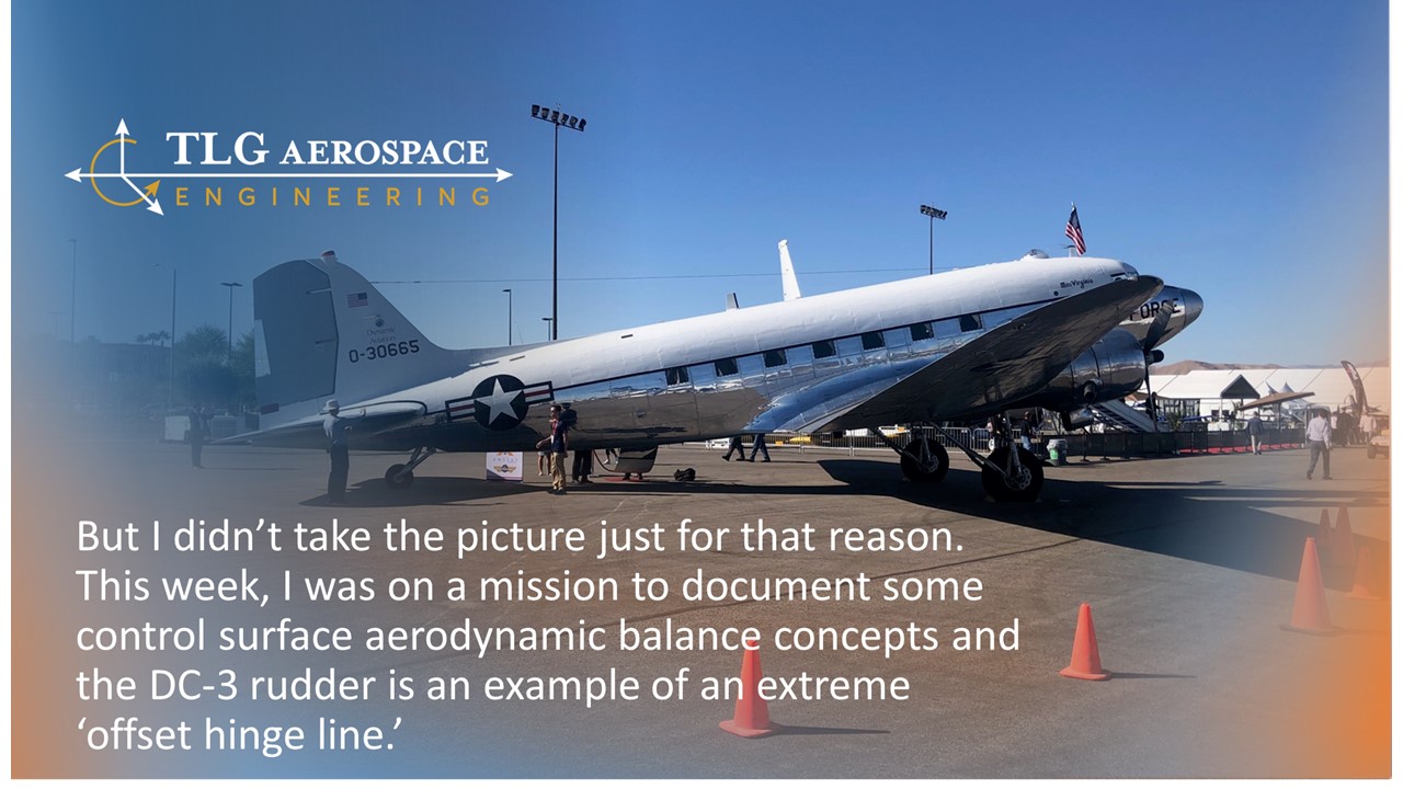
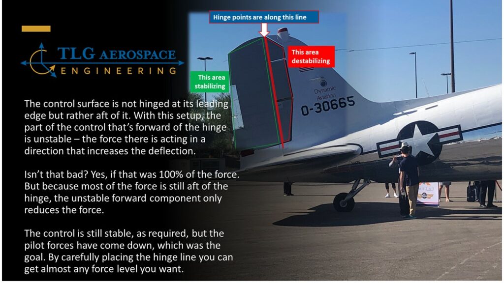
Below, Robert summarizes his mission to document some control surface aerodynamic balance concepts at the aircraft display. The DC-3 rudder is an example of an extreme ‘offset hinge line.’ Read on for more from Robert . . .


Hypersonic Flow on the X-34 with Adaptive Mesh Refinement
TLG uses the latest version of CD-adapco’s Navier Stokes Solver STAR-CCM+ for Computational Fluid Dynamics (CFD) calculations. Whenever there’s a little down time, we like to keep the solver running on problems which expand both our knowledge and our validation database for the code. One good example of this is the NASA X-34 Vehicle. The X-34 was a technology demonstrator intended to help develop the reusable launch vehicle technology by making frequent hypersonic, sub-orbital hops followed by a fast turn-around. A lot of wind tunnel testing was done on the vehicle, which unfortunately never flew after funding priorities changed.
For this CFD experiment, TLG decided to test the CCM+ adaptive mesh refinement capability at a Mach 6, 15° angle of attack re-entry condition for the X-34 and compare the resulting shock angles to the Schlieren images given in AIAA-98-0881.
Initial Mesh Generation
Normally CFD mesh generation provides maximum refinement (smallest size) only at the areas of high curvatures near the vehicle, and then the cell sizes grow with distance into the free stream. For subsonic flows, this works well and the quickly growing cell sizes keep memory and CPU requirements reasonable. This approach provides the initial mesh for the X34 as shown in Figure 1, which is a Cartesian off-body mesh with trimmed cells at the body interface.
However, for hypersonic flow there is a detached shock, like the bow wave of a boat. Since aerodynamics change very quickly across a shock (by definition), and since the propagation of the shock into the far field affects the accuracy of the solution, it will be necessary to refine the off-body mesh to capture the shock in 3D.
Mesh Refinement
In order to place more cells in the location of the shock, a CCM+ “user defined field function” was created, which marked all the grid cells in the volume solution with Mach 5.88 to 5.99 – i.e. just below the free stream Mach number. In the initial very coarse off-body grid, this results in the big blocky blue cells shown in Figure 2, which is a 2D section taken at the centerline of the volume mesh. The mesher was then re-run with a small cell size refinement dictated by the field function, the solution re-started and converged to a sharper shock in the far field. The entire process was repeated a second time to finally arrive at the off-body mesh with localized refinement along the major shocks as shown in Figure 3. Because the solution could be interpolated to the new mesh and restarted each time, the additional run times as the mesh density increased were significantly reduced from a ‘clean start’ condition.
Shock Angles and Experimental Data
The real check on the method comes with comparison to experimental data. This was done by over-laying the CFD side view against the Schlieren images published in AIAA-98-0881, as shown in Figure 4. While the CFD is a 2D slice through a 3D solution, the Schieren is 3D, but the strongest shocks are still going to be the nose in the 2D plane allowing for easy comparison to the CFD solution. The upper shock angle shows a very nice correlation with the computational result, and the lower shock angle is very close, less than two degrees difference, as shown by the red circles. The final image shows the 3D nature of the full solution by putting Mach contours on a series of six cut planes along the body.